Using Dichotomy to Teach Monetary Theory II: Demystifying Demand for Money

The logic of an inflation driven by money printing is intuitive. If you print more money, the prices of goods purchased with it will tend to rise. However, the idea that there is a demand for money is not so intuitive. Money is half of every transaction, so it is clear that people demand it. But does demand for money change? And, if so, how can we describe the change?

In the last post, I used the equation of exchange to derive the aggregate-demand curve. We defined the equation of exchange:

MV ≡ Py

The equation of exchange also provides building blocks for understanding the dynamics of the market for money. Last time, we adjusted the quantity of money, M, to show the influence of changes in the quantity of money on the goods market. Since aggregate demand (total expenditures) is defined by the product of M, the quantity of money, and V, the average rate at which each unit of money is spent, an increase in M is associated with an increase in aggregate demand. We could have shown that an increase in V can lead to the same outcome. In the remainder of this post, we will see that changes in the velocity of money represent changes in demand to hold money. We will also consider a second form of demand for money: demand to spend money.

Demand for Money and the Equation of Exchange

The equation of exchange, in its standard form, shows that aggregate demand (MV) must equal the nominal value of aggregate supply (Py). If we rewrite the equation, we can show that the quantity of money supplied must equal the quantity of money demanded:

M ≡ Py/V

Velocity, the average rate at which each monetary unit is spent, is simply the inverse of demand to hold money (k). Thus:

M ≡ Pyk

We identify the motives for demanding money as demand to spend money (transaction demand) and demand to hold money (portfolio demand). Demand to spend money is Py, nominal income, and demand to hold money is k, the inverse of velocity.  In equilibrium, the quantity of money supplied to the market must equal the quantity of money demanded. For now, we will assume the quantity of money is held constant.

Demand for Money and the Price Level

What I refer to as demand to hold money is traditionally referred to as portfolio demand for money. This is a long-run demand to hold money. For example, let’s assume you prefer to hold onto $1,000 of cash at all times. If you ever spend this reserve, you will quickly rebuild it. Every dollar removed from circulation in the effort at rebuilding tends to reduce velocity, V. Thus, a fall in V necessarily implies a rise in this long-run level of demand to hold money, k.

It might appear that if demand for money increases, the quantity of money must increase. This is not necessarily true. An increase in demand for money, for example, can be offset either by an increase in the money stock or a general fall in prices. We can rearrange the equation of exchange to reflect this:

M/P ≡ yk

In monetary theory, we refer to yk as demand for real cash balances. This is a fancy way of saying we can adjust our measure of the money stock for inflation.

The simplest model of the market for money assumes the quantity of money will not adjust to changes in the price level. In the very short run, this is true, and thus a convenient approximation of reality. Either an increase in demand to hold money or an increase in demand to spend money is represented identically in the graph of the market for money:

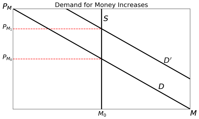
If we relate this to the equation of exchange, we see that an increase in demand for money is associated with an increase in the price of money, PM. We expected that an increase in demand for money would be associated with a fall in the price level. The increase in the price of money implies exactly this since, as we observed in the last post in this series, PM = 1/P.

Demand for Money and the Goods Market

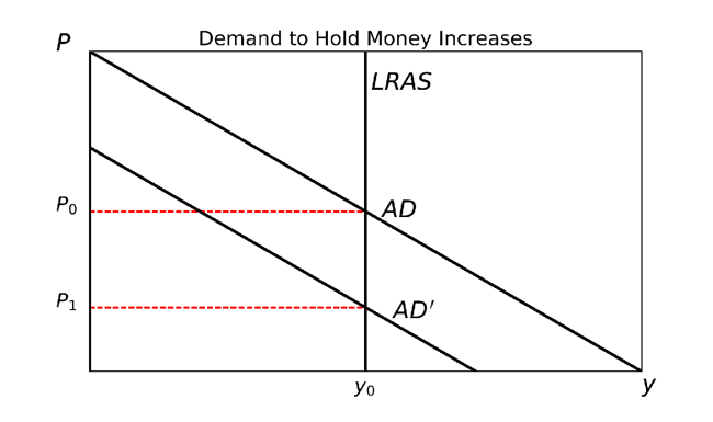
The two different types of demand for money represent two different processes in the goods market. In the case in which demand to hold money increases, we refer to this as an autonomous decision on the part of money holders. They simply have adjusted their preference for money as compared to other goods. If, on average, individuals decide to hold more money on reserve, meaning V has fallen (k has risen), this means less money is available for expenditure on other goods. Since there has been no change in the quantity of money or other goods available, this requires that the price level (P) fall.

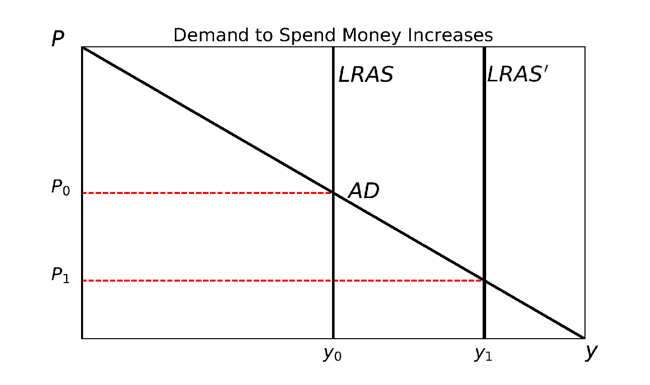
Compare this to the case where demand to spend money increases. Individuals have not changed their preference to hold or even to spend money. Rather, there has been a change in the environment. More goods are available for purchase. Consumers who would like to buy these goods find themselves unable so long as prices do not fall. Thus, an increase in demand to spend money must lead to falling prices so long as the quantity of money is unable to adjust.

The following representations of the market for non-money goods are associated with the increases in demand for money mentioned above:

So far we have only considered cases in which the quantity of money, for reasons either of time or institutional structure, is unable to adjust to changes in demand for money. In these cases, it is necessary for prices to be capable of adjusting quickly to reflect changes in demand for money. Policies that tend to make prices inflexible — legally binding minimum or maximum prices — inhibit this adjustment of prices and can increase the length and severity of depression. In like manner, policies that prevent the adjustment of the money stock to changes in demand for money also generate macroeconomic disequilibrium.

In the next post, we will develop our analysis to include markets for money and credit that are responsive to changes in demand for money.

Related Articles – History