Using Dichotomy to Teach Monetary Theory

Monetary theory is beautifully simple, although to the uninitiated it may seem terribly complex, especially if you are not acquainted with the fundamentals of economic decision-making. Humans economize, attempting to reduce costs and maximize the value that results from their actions. This fundamental principle underlies decisions to hold money or goods and what form of money to hold. Once you understand the logic of economic theory, you are ready to appreciate the simplicity of monetary theory.

In class, I attempt to convey this simplicity through exploring three dichotomies:

1. In a money economy, analysis of economic activity can be divided between money and non-money goods.
2. Money has value because people demand it. This demand can be split between demand to hold money and demand to spend money.
3. The quantity of money can also be divided into two categories: base money (such as gold in a gold-standard economy) and credit money (what Ludwig von Mises referred to as fiduciary currency).

As individuals choose between the options presented by these dichotomies, their actions tend to be driven by changes in the costs of choosing one option or another. Over the course of this series of posts, I will show the usefulness of these dichotomies for presenting macroeconomic dynamics to students.

Today, let’s consider the macroeconomic dichotomy between money and non-money goods. Changes in the market for money effect changes in the goods market and vice versa. For example, if the quantity of money increases, the nominal (i.e., not adjusted for inflation) value of total expenditures also increases.

While a simple narrative can link together the markets for money and non-money goods, a brief description is necessarily incomplete. Macroeconomic theory systematically links these two markets in the equation of exchange. The equation is an identity that affirms that at all times, total expenditures must be equal to the total value of goods purchased in the market. We formally express the equation of exchange as follows:

MV ≡ Py

From left to right, this says that, over a period of time, the quantity of money (M) times the average rate of expenditure of each unit of money (V) is equal to the nominal value of goods purchased (Py). We typically refer to this last value as nominal income.

If there is $1 million in circulation and each of these dollars is spent on average three times, then M times V is $3 million. The right-hand side of the equation reduces goods to a unit of real (i.e., inflation-adjusted) value (y) and the average price of a unit of real value (P).

The presentation divides the macroeconomic world between the demand side of the economy and the supply side. Since money is required to effectively demand goods, we say aggregate demand is equal to MV. Aggregate demand is the value of total expenditures in the economy. In the above example, we would say that aggregate demand equals $3 million. Aggregate demand (MV) always equals aggregate supply (Py). In equilibrium, aggregate supply reaches its sustainable long-run value.

The model assumes that in the long run, prices will adjust such that all available goods will be purchased. In other words, markets clear. Now suppose the money stock increases from $1 million to $2 million and velocity remains constant. Total expenditures would now equal $6 million. However, there is no reason to expect the economy will be able to sustainably produce more goods. Increased expenditures will force up prices of goods until the economy returns to a stable level of output.

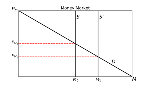
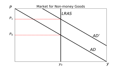
We represent this process with graphs of the markets for money and non-money goods. An increase in the quantity of money (M) leads to an increase in aggregate demand (AD). Thus, we shift the money-supply curve to the right and show the response of the AD curve, which also shifts to the right.

If prices of non-money goods do not immediately rise, consumers are able to purchase more goods than can be sustainably produced (i.e., we are to the right of the long-run aggregate-supply curve (LRAS). Prices must rise as increased consumption bids up the prices of final goods and the prices of their inputs. This moves the goods market to a new equilibrium price level of P₁. Notice that the increase in the quantity of money is also associated with a fall in the price of money, P_M (=1/P). The lower price of money associated with the new price level is P_M1. This coheres with our intuition that a fall in the value of the monetary unit is associated with a rise in prices of non-money goods.

In the next post, we will consider the dichotomy of demand for money, modeling the different effects of changes in demand to spend money and demand to hold money.

Related Articles – Economic Education