The Fatal Conceit of COVID-19 Epidemic Models


With apologies to Friedrich Hayek, I find there is a fatal conceit amongst purveyors of epidemiological information that imply they know more than they can know when forecasting the outlook for a new infection. Of course, we have to do the best we can with limited information, but we should be humble in forecasting and reluctant to support politically inspired prescriptions of how society and the economy should be regulated in the face of uncertainty. We have to be very conservative because, more often than not, the first words out of a politician’s mouth is “what’s the worst case?” From that answer comes policy recommendations.
Be skeptical in the following sense. Long ago the great Austrian economist, Fritz Machlup, observed that in order to understand an economist (you can substitute the word ‘scientist;’) you need to know what interests he serves. For example, an economist from the chemical industry is unlikely to say anything negative about the outlook for that industry. So, it can be true for scientists due to the influence of funding sources they depend on.
Basic Model
Ever since the modelling work of Kermack and McKendrick in 1927, the mathematical description of how epidemics spread has grown in complexity, but the basic form remains the same. Below is described the five most basic equations that are extensions of their original work. It will be kept simple, but there is a major point to be made that is best understood if one has some understanding first of the equations used.
The key to validity is not the form of the equations, but the parameters to the equations. In early days those parameters need to be estimated with sparsely available data; therefore it is easy to reach conclusions that depend less on the certainty of facts than on the assumptions made. You get what you assume rather than getting what is justified by the facts to become known. Massage the input parameters and you get the outputs you desire. Recall the advice of Machlup.
The use of symbols is not to impress but to provide a sense of what we are talking about in a structured way. The first four equations are differential equations that describe the non-linear path of progression (in units of daily change). Specifically, they describe the propagation of an infection as it works its way through a population causing people to transition between four states starting with S, those that are susceptible, to E, those who are exposed, to I, those who are infected (also described as those who are infectious) and finally, R, those who have recovered. The states and the transitions from one to the next are pictured this way:
St(susceptible) ➞ Et(exposed) ➞ It(infected/tious) ➞ Rt(recovered)
The changes (that’s what ∂ means) in the number of people in each state per unit of time is described as follows:
1. ∂S/∂t = µN – µS – β SI/N
2. ∂E/∂t = β SI/N – (µ + α)Ε
3. ∂I/∂t = α E – (γ − μ)Ι
4. ∂R/∂t = γΙ − μR
5. Rο = α/(μ+α) * β/(μ+γ)
The trajectory of the growth in deaths is derived indirectly by the difference between the infected (I) and the recovered (R).
The number of people in each group varies over time as people transition from group to group according to the probability of contact with someone who is infected, the probability the contact will result in an infection and the probability they will recover from the infection. The ‘Greek’ symbols are expressions of the transition probabilities and have the following meaning:
β = contact rate, i.e., the average number of contacts of a susceptible person per day, that is sufficient for disease transmission.
µ = mortality rate (% of group)
α = 1/average incubation period (as a % of a year)
γ = 1/average infectious period (as a % of a year)
The R-Naught Bugaboo
The 5th equation shows the calculation of a single number, the dreaded “reproduction number.” Also referred to as R naught, it is the number of people that one person – that is, the first person to contract the disease – will infect at the onset of the disease. (Notice the letter R is in bold italics, so as to distinguish it from R, the number of recovered patients).
R naught was made popular in the movie Contagion, so a large number of people have a passing familiarity with the concept. In the movie and in life there is a lot of anxiety over the correct value of R naught because in the movie it would determine the fate of mankind in the absence of a cure.
In fact, R naught (Ro) is not directly measured. No one knows how many people were infected by the first infectious person. So, it has to be estimated as a point estimate, meaning it is a single number; that is derived from other numbers, which are themselves inimical to driving the entire hypothetical disease propagation. Though it is an initial condition which determines the behavior of the spread of an infection from the onset we will never directly measure it. It is very important that Ro and its confidence interval are estimated as accurately as possible. However, several other equation parameters come into play, which they themselves are also estimated, and greatly affect the course of an epidemic.
An even bigger question, left unanswered in most academic papers you may read, is how did they come by this simple equation for Ro? Can it be observed directly or is it the byproduct of calculations solving the integrals for the differential equations 1-4, to determine the steady state outcome from initial assumed values of the parameters? This latter approach results in a so-called reduced-form derivation. Since, in the real world for a new disease, most of the parameters (the ‘Greeks’) are unknown, a simulation can be run based on early tracking to estimate the parameters. Those estimates are improved upon over time as more data is obtained. Once the steady state outcome is calculated from the initial assumptions, a contact number, Ro, can be backward-derived. Many simplifying assumptions are made along the way.
In early days epidemiologists can try to estimate R0 using contact tracing data obtained at the individual level. Who was the first to infect others is uncertain, so you search for the earliest patients who were diagnosed as infected. Their contacts are traced backward and each tested. R0 is then computed by averaging the results for many diagnosed individuals. It is a crude approach.
The other approach is to obtain R0 from cumulative data. This involves making assumptions based on ordinary differential equations that describe the dynamics at the population level of the number of people in each state without actually tracking specific individuals. It is very important to note that one method cannot be used to validate the other method. Mathematically, the relationship between the two calculations is considered complex and unknown.
From this point forward there is no need to further reference the differential equations 1-4 shown above. Instead, the focus will be on the calculation of the dreaded Ro. It is derived from four other values that are unknown at the onset of a new disease such as COVID-19. In fact, these values are not only difficult to estimate, but two of them are sure to change over time as the infected population adjusts to the reality of the infection. So whatever value is initially assumed for Ro it is sure to change over time as well as with better data.
But here is the odd thing. The convention amongst epidemiologists is to leave Ro unchanged; it is considered a ‘threshold’ value. It is kept constant. They know that once over the ‘threshold’ the reproduction rate will ‘evolve’ but they call it something else. Furthermore, as will become clear from examples given below, very small errors of measurement of the inputs to the calculation of Ro will have very large effects on the estimated “reproduction number” Ro.
It becomes obvious that any shortcomings in the objectivity and reporting of the early estimates of Ro can set off considerable fear and therefore likely result in wrong-headed personal and policy responses.
Early Estimates of Ro
Health department spokesmen have given enormous emphasis in the press to the reproduction number Ro. It is treated with reverence and fear because, all other things being equal, if it is greater than 2 the infection can rapidly spread and lead to very high infection and death rates.
It seems like such a simple number with such high certainty attached to it. It is used in a way that it can be compared to the pass accuracy rate of a football quarterback. So-and-so has a 98% pass accuracy. But anyone who follows the game knows that you need to know a lot more if they are going to gain yardage on the field. You need to know if the intended receiver catches it, fumbles it, is bumped off, or it is intercepted. Just as it is true that you need to know more variables than just pass accuracy, it is equally the case for a disease. But it is even harder because a new disease is a one-time thing; it has no history. The rate of spread and lethality will not be known accurately until the end of the disease’s propagation. As in football, there are defenses against an accurate passer, so is it true that many things will affect the course of a disease other than simply the Ro.
What have we been told about COVID-19’s Ro?
- An early study for the CDC by a group of scientists at Los Alamos, using Chinese data, estimated Ro at 5.7 with a confidence interval of 3.8 to 8.9. A frighteningly high number.
- A later study based on data from Italy put the Ro at 2.43 to 3.10.
- In another study a Harvard scientist suggested Ro was in the 5 to 6 range.
For further perspective, calculations of Ro for Rubella (German measles) was 6.4, for mononucleosis 2.2, for H3N2 (Hong Kong flu) 1.44 and for H2N2 (the Asian flu) 1.33.
Keep in mind that if Ro is less than 1 there will not be an epidemic. It will die out quickly. If it is greater than 2 it is a very serious epidemic.
At this point serious work is no longer focused on estimation of the threshold value of Ro. That is considered yesterday’s problem and it doesn’t matter anymore, even if the estimate was wrong in the first place. Furthermore, the reproduction rate declines naturally anyway since the contact rate will decrease as the number of recovered cases increases thus reducing the number of people who can still be infected. Today the focus of politicians is to further reduce the reproduction rate by social engineering; that is, to force a reduction in contacts between the susceptible by social distancing.
Also, keep in mind that Ro is a ‘statistical on average number.’ It can have about as much meaning as the statement that you will not drown crossing a river with an average depth of 3 feet. We all know how that can go wrong. At the individual level, the number of contacts vary widely based on age, region, occupation, etc. For example, for some spreaders (infectious people) the initial reproduction rate might be 12 and for others 0.
Even more important to the outcome of a disease is the recovery rate and the susceptibility rate. Those two factors are also not known until after the fact. Whether exposure will lead to an infection depends on the precautions taken on both sides of social intercourse. That is why people are encouraged to be extra careful in their sanitary habits because that likely will result in a significantly lower infection transmission rate.
As for the susceptibility rate, most epidemiologists assume that some portion is likely to have some sort of natural immunity. They can’t be sure. They start with a zero assumption but as time goes on it is often discovered that exposure to some other disease has given some people an immunity or a decreased susceptibility to the new disease.
Homemade Estimates of Ro
OK, let’s look at what goes into the estimation of Ro. From equation 5 (repeated below for convenience) we see that α, β, μ, and γ went into the calculation.
Recalling the reduced-form formula derived from the four partial derivative equations, and the parameter definitions:
Rο = α/(μ+α) * β/(μ+γ)
β = contact rate, i.e., the average number of contacts of a susceptible person per day, that is sufficient for transmission.
µ = mortality rate (% of group)
α = 1/average incubation period (as a % of a year)
γ = 1/average infectious period (as a % of a year)
Notice there is a circularity in the calculation. At the get-go we need as an input the death or mortality rate (µ). It is certainly a very important number to know, but we won’t know it until the epidemic has played out. The average infection period (γ) can be observed and averaged across patients if you know when the infected person became infected and how long it took for him to not be infectious. It means a lot of daily tests. The incubation period (α) can also be measured if you know when they were exposed and when they came down with symptoms. Finally, there’s the contact rate (β). That too is a guess. The contact rate is a number that estimates the average number of contacts a susceptible person experiences in a day that is sufficient for the transmission of the disease. It is not the total number of contacts one has but only that subset with those who are infectious and that those contacts must be serious enough that there could be transmission.
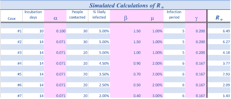
First, let’s make some guesses at each parameter to get a feel for magnitudes and sensitivities. The values used in each of the cases described next are also recorded in the Table below.
Case #1
Assume the average incubation period is 10 days, then α is 0.1.
Assume a susceptible person comes into contact with 30 people in a day and 5% of them are infected and in close enough contact to cause transmission. Then the contact rate β would be 1.5.
Further, assume the mortality (death) rate, µ is 1%.
Finally, assume the infection period is 5 days, then γ is 0.2.
Solving for Ro we get:
Ro = .1/(.01 + 0.1) x 1.5/(.01 + 0.2)
= 0.1/0.11 x 1.5/0.21
= 0.909 x 7.143
= 6.49
That value is similar to the early estimate based on Chinese data cited earlier.
Case #2
Evidence suggests the incubation period may be somewhat longer, e.g., 14 days. That causes Ro to decrease slightly to 6.27.
Case #3
If the number of contacts ‘susceptibles’ have with people who are infected, and where the contact is significant at 5%, drops to 20, then Ro falls to 4.18.
The remaining 4 of the 7 cases show different combinations of assumptions of the parameters. Primarily the infection period is lengthened and the likelihood of an infection from a contact is reduced. By the 7th simulation, the initial estimate of Ro drops to below 2.
Conclusion
The epidemiological world has published countless articles and studies warning against the tendency and ease with which one can overestimate Ro. We have fallen prey to this tendency once again. The Fatal Conceit of bureaucrats in the service of politicians is that they imagine they know more than they actually need to know to design appropriate policy. They employ many scientists who struggle to maintain objectivity, but it is easy for those who control their budgets to pick and choose whose work they will support. Small errors of assumptions can produce large errors of policy.
When it is argued that it is “better to be safe than sorry,” the response should be “how do you measure the value of ‘safe?’” Number of sick, number of deaths, loss of freedom, loss to the economy? Is a loss of profits or GDP ever worth more than the loss of a life?
In war a general can ask for people to risk their lives for an objective. In peace time that ask can never be made.
The best answer would be to allow freedom of choice; that is, people should be granted the freedom to pursue personal preferences and arrangements. That freedom will result in manifold decisions. If left to the politician there will be only one decision, one that most assuredly will lead to a loss of personal and economic freedom.
Gregory van Kipnis