An Inflation Primer
Inflation, broadly defined, is growth in the general level of prices. The federal Bureau of Labor Statistics publishes a monthly measure of aggregate consumer price changes—the Consumer Price Index, or CPI. Growth in the CPI is usually called CPI inflation. The Federal Reserve, the central bank of the U.S., is mandated to promote price stability, along with full employment. It uses another inflation gauge, the personal consumption expenditure price index, called PCE inflation.
In narrow terms, inflation can refer to inflated prices for specific items. The average sales price of new homes sold in the U.S. was $360,600 in 2015, up from $345,800 in 2014, according to U.S. Census Bureau. In this case, the annual inflation rate in the price of new homes in 2015 was about 4.3 percent.
While buyers and sellers have different views on inflation, the Fed has a target inflation rate of two percent, not zero. That level is also targeted by central banks in other developed countries. Hyperinflation, on the other hand, has proved costly to economic growth.
Inflation is critical to individuals’ decision making
Since inflation is the price growth of everything from groceries and housing to education, it is part of everyday life, so it is a critical consideration in personal decision making. Consumers who expect a higher inflation rate in the future would have an incentive to make purchases now rather than later. A home buyer would rather buy a house now if he or she believes the average home price would grow by 4.3 percent next year.
Inflation is also fundamental to savers, who need to be aware that their savings have less purchasing power with inflation. The $5,000 saved by a grandmother will be worth less in the future if she hides the money in the toilet tank or under her bed. And if the inflation rate is 2 percent, a 1 percent interest rate earned on savings accounts will not make up for the loss in purchasing power caused by inflation.
For investors, inflation matters in assessing the profitability of projects. A project with a 5 percent expected rate of return would make sense if the inflation rate was 3 percent. But if future inflation of 10 percent is expected, the project would fall apart. For long-term investments, inflation may be even more important. Most long-term projects require a large capital investment in the beginning, usually referred to as sunk costs. However, it is more difficult to accurately forecast inflation in the long term than in the short run.
How hyperinflation hurts the economy
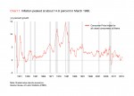
The next question, naturally, is whether hyperinflation in the U.S. has ever occurred, damaging consumption, savings, and investment. The answer is yes. Chart 1 shows year-over-year CPI inflation in the U.S. from January 1948 to March 2016.
The history of U.S. inflation shown in Chart 1 is nothing like Zimbabwe’s, where monthly inflation reached about 80 billion percent at the end of 2008. But some periods of high U.S. inflation have been costly to the economy. The Great Inflation of 1965–1984 and a stagflation crisis in the late 1970s are still vivid memories. Stocks crashed, losing half of their value, and the unemployment rate in the early 1980s almost reached double digits.
The Great Inflation was blamed on oil crises, policymakers’ errors, and the dysfunction of economic theories. Simple Keynesian models were thought to be at fault, for example. Specific factors may have contributed to the abnormal inflation hikes, but throughout the entire history of our fiat money system, (in which the government declares currency as legal tender), inflation has existed most of the time. So what causes it?
In the long run, money is at the root of the matter
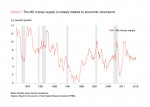
When abundant money is chasing limited goods or services, inflation occurs. In the current fiat system, the central bank can create money without it being backed by any physical commodities. Since the early 1970s the U.S. dollar has no longer been tied to gold and has become a fiat currency. Between January 1972 and March 2016, the U.S. money supply increased from $718 billion to $12.6 trillion by the M2 money measure, which includes cash and checking deposits (known as M1) plus other monetary assets that can be quickly converted into cash. Chart 2 shows the year-over-year growth of M2 in 1972– 2016.
As Chart 2 shows, the M2 money supply skyrocketed in the 1970s (it grew by double digits for years), resulting in high inflation. High money supply growth often has caused high inflation, coinciding with economic downturns, such as in 1990, 2001, and 2009.
In the past several years, the M2 money supply has been growing modestly at a range of 5–6 percent a year. In consequence, inflation has been sluggish. Going forward, however, there is a risk of high inflation. Abundant liquidity was created as a result of the Fed’s quantitative easing programs from 2008 to 2014. There is now $2.4 trillion sitting in the banking system as excess reserves. That accounts for about 19 percent of the current M2 money supply (or $2.4 trillion of the $12.6 trillion in M2). If all that money was loaned out and all else held equal, there would be 19 percent inflation immediately.
On the other hand, in the short term, price growth (i.e., inflation) is most likely affected by demand and supply. We learned in Econ 101 that higher demand results in higher prices. On the other hand, higher supply leads to lower prices. But in the longer run, supply would adjust in response to the change in demand, pushing the price back to the pre-change level.
Our new inflation forecasting model tests well over three decades
Since inflation is not only crucially important to economic growth but also to individuals’ economic wellness, inflation forecasting has attracted a lot of attention. But there is a shortage of forecasting models that perform well. The Phillips Curve framework, which assumes a trade-off between unemployment and inflation, has been widely used. But when double-digit unemployment and hyperinflation co-existed from the late 1970s to the early 1980s, that framework fell apart. Since then, it has received much criticism.
At AIER we conducted a time-series analysis to improve the performance of short-term inflation forecasting. We focused on the short term rather than long term for two main reasons. First, a short-term inflation forecast provides individuals with a useful perspective on price growth in the near future. It helps them make better decisions about purchasing, saving, and investing, to improve their economic wellness. Second, any time-series analysis is based on one fundamental assumption: that economic structures don’t change over time. But this isn’t really the case. Restricting time-series models to predicting the near future and updating the models on a regular basis help minimize the gap between assumption and reality.
Our forecasting model, developed over the past year, consists of three procedures. In step 1, we ran statistical tests on various economic variables (monthly from 1960 to 2015), including labor-market conditions, consumer demand, supply of goods and services, money supply, interest rates, stock indexes, and housing. The test results showed whether each variable could predict core-CPI inflation (core CPI excludes volatile food and energy prices). Based on the results, seven variables were selected (Table 1).
In step 2, we applied the seven variables in an advanced econometric model, called a dynamic-factor model, to capture one factor that would represent all seven variables. This is an essential procedure for improving the performance of a time-series analysis in forecasting inflation. It is like a pre-cooking step, extracting a concentrated broth from different ingredients. The broth can be used later to substantially improve taste of the final dish.
In the final step, we constructed a time-series model to forecast inflation. There are two predictors in the model. One is lagged core-CPI inflation. The other is the factor from Step 2 that represents the seven selected economic variables.
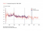
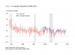
In order to test the performance of the model, we performed several forecasts for different periods of time in the past. This is usually called in-sample forecasting. Chart 3 gives the in-sample forecast result for 2005–2015, and Chart 4 shows a forecast for 1985–2004.
The results show that our monthly forecast for the past decade was, on average, 0.05 percent greater than the actual inflation rate. This means if actual core CPI inflation was 0.50 percent in December 2015, our forecast would most likely be about 0.55 percent.
Our forecast for 1985–2004 exceeded the actual inflation rate during the same period by 0.02 percent on average. This means if the actual core CPI inflation was 0.50 percent in March 2000, our forecast would most likely be about 0.52 percent. Compared with the scale of historical monthly core-CPI growth, both of our forecasts diverged only slightly from the actual data.
We then ran the model (using all the available data up to April 2016) for monthly core-CPI inflation forecasts for the following six months. It predicts that the average monthly core-CPI inflation in the next six months will be in the range of 0.14 to 0.17 percent.
Note that time-series forecast models do not take into account unexpected situations. For example, apparel prices jumped 1.6 percent in February 2016, their biggest monthly gain in seven years. Then they tumbled 1.1 percent in March. So it is hard to predict where the data will show apparel prices are headed in the near future and how they will affect core-CPI monthly growth. The forecast results assumed that the trend from the previous months would continue for the months ahead. Any unexpected events would jeopardize their accuracy.
The inflation forecasts for the next six months show a rather flat trend. This is in line with the sluggish price growth over the past few years. For consumers, there is no reason to rush in making purchases. For savers, this is obviously good news, since low inflation means less of a reduction in the purchasing power of their savings. For investors, projects are likely to be more profitable with a low inflation rate, if all else holds equal.
The low likelihood of a big change in inflation could also ease policymakers’ concerns about high future inflation, at least for the months ahead. It may reassure the Fed that it can proceed slowly in raising interest rates for the rest of the year.
Takeaways
In the short term, demand and supply of goods and services are the main drivers of price growth.
In the long run, an abundant money supply causes inflation.
Short-term forecasting is likely to be more accurate than long-term inflation projections based on a time-series analysis.
The U.S. economy may be exposed to the risk of future high inflation due to enormous excess bank reserves.
In the short term, inflation will continue to be mild, according to the forecasts.


